

Appearance
Quantification Methods
What this is
This page gives the details of each risk quantification method in Modulos. Each method gives one monetary expected loss. Modulos uses this value for the totals, the limits, and the priorities.
For the model and the workflow, see Risk Quantification.
Where in Modulos
Select the method in the quantification wizard:
AI System → Risks → [Risk] → Threat Vectors → Quantify → Select Method
After you select a method, the Configure Parameters step shows the fields of that method. The result shows on the Current Analysis tab of the Threat Quantification Detail page.
Who can do what
Only users who can quantify threats can open the wizard. See Risk Quantification.
At a glance
Each method, what it does, and when to use it:
| Method | What it does | When to use it |
|---|---|---|
| Risk Agent | An AI agent makes a Fermi estimate from the data of the AI System, and records its assumptions. You enter nothing. | A first estimate that a person then examines |
| Manual Entry | Records a monetary value and an optional description | Fast: you have a number that you can defend |
| Scenario Analysis | Calculates the expected loss from three scenarios, each with a probability and an impact | Recommended default: you start without incident data and want clear assumptions |
| Monte Carlo Simulation | Simulates many years of losses from a loss range and a frequency, and gives the expected loss and the tail | Advanced: you want a probabilistic model and can defend its inputs |
| Risk Matrix | Changes a likelihood score and an impact score into money with a scaling factor and a frequency multiplier | Only when you have a calibrated mapping from scores to money |
Manual entry
Use Manual Entry when you have a monetary estimate that you can defend, and you want to record it quickly.
Inputs
value: the monetary expected loss in the currency of your organization. The API accepts 0, or a number from 0.01 to 10,000,000,000,000.description: context, assumptions, or the source of the estimate, as a string ornull. The request must contain this key.
UI fields
- Value: necessary, from 0.01 to 10,000,000,000,000.
- Description: optional.
API payload
json
{
  "method": "manual_entry",
  "value": 2400000,
  "description": "Expected annual loss based on incident history and remediation cost."
}Result: the Manual Entry Details panel shows the Entered Value and the Description.
Notes
- Use the number as a model output, not as a rating. Record the assumptions in the description. Then other persons can examine them.
- Use the same time basis as your risk appetite. In most organizations, this basis is one year.
Scenario analysis
Scenario Analysis is the recommended default method when you want a clear structure without a complex model. It makes you write clear assumptions. It calculates a monetary expected loss from a set of scenarios.
Formula
text
Expected loss = Σ (probability × impact × (1 - mitigation_effectiveness) × weight)This method is deterministic: the same parameters always give the same output.
Inputs
scenarios: a set of scenarios.name: a necessary identifier for reports.probability: the likelihood of the scenario, in[0, 1].impact: the monetary loss when the scenario occurs,>= 0.mitigation_effectiveness: the fraction of the impact that mitigation removes, in[0, 1].weight: a positive multiplier for the scenario,> 0.
normalize_weights: whentrue, Modulos scales the weights to a sum of 1.strict_probabilities: whentrue, the method makes sure that the scenario probabilities have a sum of 1, in the tolerance.probability_tolerance: the permitted difference from 1 when the strict check is on. The default is0.05.
UI fields
In the wizard, Scenario Analysis has three rows: Best Case, Worst Case, and Base Case. Each row has these columns:
- The Probability column: a number from 0 to 1, with a slider in steps of 0.1.
- The Impact column: the monetary loss of the scenario. The minimum is 1.
- The Contribution column: the Probability multiplied by the Impact, and its percentage of the total. Modulos calculates this column.
The wizard does not send mitigation_effectiveness or weight. The method then uses 0 and 1.
Result: the Scenario Analysis Results panel shows each scenario with its contribution, the Weighted Expected Value, and the Range. When a scenario has a mitigation, the panel also shows the Residual Risk, the Mitigation, and the value Before Mitigation. A Key Assumptions section follows.
API payload
json
{
  "method": "scenario_analysis",
  "scenarios": [
    { "name": "best_case", "probability": 0.2, "impact": 200000 },
    { "name": "base_case", "probability": 0.6, "impact": 1200000 },
    { "name": "worst_case", "probability": 0.2, "impact": 7000000 }
  ]
}
Probability hygiene
By default, Scenario Analysis runs also when the sum of the probabilities is not 1. If the difference from 1 is more than the tolerance, the method records a warning in the output. Turn on strict probabilities only when you want Modulos to refuse inputs that do not agree.
When to use
- You start without incident data and want a clear model that other persons can examine.
- You want leaders to see the assumptions: what can occur, how likely it is, and how much it costs.
- You want a stable baseline that you can make better when you get more Evidence.
Frequent errors
- Probabilities that are only feelings, and not clear claims that other persons can examine.
- Best and worst cases that are only "optimistic" and "pessimistic", without impacts from actual cost drivers.
Monte Carlo frequency and severity
Monte Carlo Simulation simulates many years of losses from your estimates of loss and frequency. It gives the expected annual loss and the tail metrics: quantiles, VaR, and CVaR.
Modulos has two models:
probability_impact: one incident can occur in a period, with the probabilitypand an uncertain severity.frequency_severity: many incidents can occur in a period, with an uncertain frequency and an uncertain severity.
Model: probability × impact
Use this model when the threat is one type of incident for each period. The primary uncertainty is if the incident occurs and how much it costs.
Inputs
model:probability_impactp: the probability of the incident in the period, in[0, 1]severity: the loss of one incident, as afamilywith itsparamstrials: the number of simulation trialsrng_seed: an optional seed to get the same result again
API payload
json
{
  "method": "montecarlo_frequency_severity",
  "model": "probability_impact",
  "p": 0.15,
  "severity": {
    "family": "lognormal",
    "params": { "family": "lognormal", "mu_log": 12.0, "sigma_log": 0.9 }
  },
  "trials": 10000
}
Model: frequency × severity
Use this model when the threat can occur more than one time in each period. Examples are policy violations or safety incidents that occur again.
Inputs
model:frequency_severityfrequency: the number of incidents in one period, as afamilywith itsparamsseverity,trials, andrng_seed: as in theprobability_impactmodel
API payload
json
{
  "method": "montecarlo_frequency_severity",
  "model": "frequency_severity",
  "frequency": {
    "family": "poisson",
    "params": { "family": "poisson", "lambda": 2.0 }
  },
  "severity": {
    "family": "lognormal",
    "params": { "family": "lognormal", "mu_log": 11.7, "sigma_log": 1.1 }
  },
  "trials": 50000,
  "rng_seed": 42
}
Distributions available in the platform
Each severity and frequency object in the API has this structure:
json
{
  "family": "lognormal",
  "params": {
    "family": "lognormal",
    "mu_log": 12.0,
    "sigma_log": 0.9
  }
}
Supported families:
deterministic:valuebernoulli:ppoisson:lambdalognormal:mu_log,sigma_log
The wizard uses a lognormal severity, and a Bernoulli or a Poisson frequency. For the other families, use the API.
UI fields
The Configure Parameters step of Monte Carlo Simulation has three panels and one section of settings:
- Loss magnitude: Credible low and Credible high, the loss of one incident. Modulos fits a lognormal severity distribution with these two values at the 5th and the 95th percentile. The two values must be more than 0, and the low value must be less than the high value.
- Severity preview: the loss curve of one incident from your two values, with Implied median, Implied mean, Severity p95, and Severity p99. A message shows when the tail is heavy (
sigma_logmore than 1.5). - Frequency: a switch with Once at most and Multiple times.
- For Once at most, type the Annual probability, from 0% to 100%. Modulos uses the
probability_impactmodel with a Bernoulli frequency. - For Multiple times, type the Expected events per year, more than 0. For example, 0.5 means one incident in two years. Modulos uses the
frequency_severitymodel with a Poisson frequency.
- For Once at most, type the Annual probability, from 0% to 100%. Modulos uses the
- Advanced simulation settings, closed by default: Number of trials from 1 to 100,000, with 10,000 as the default, and Random Seed. Keep Random Seed empty to get a random seed.
The wizard always requests the metrics EL, STD, QUANTILES, VAR, and CVAR. The other parameters below are available only through the API. A banner shows when you open the wizard again for a run with a different severity family or frequency family. Then type the values again.
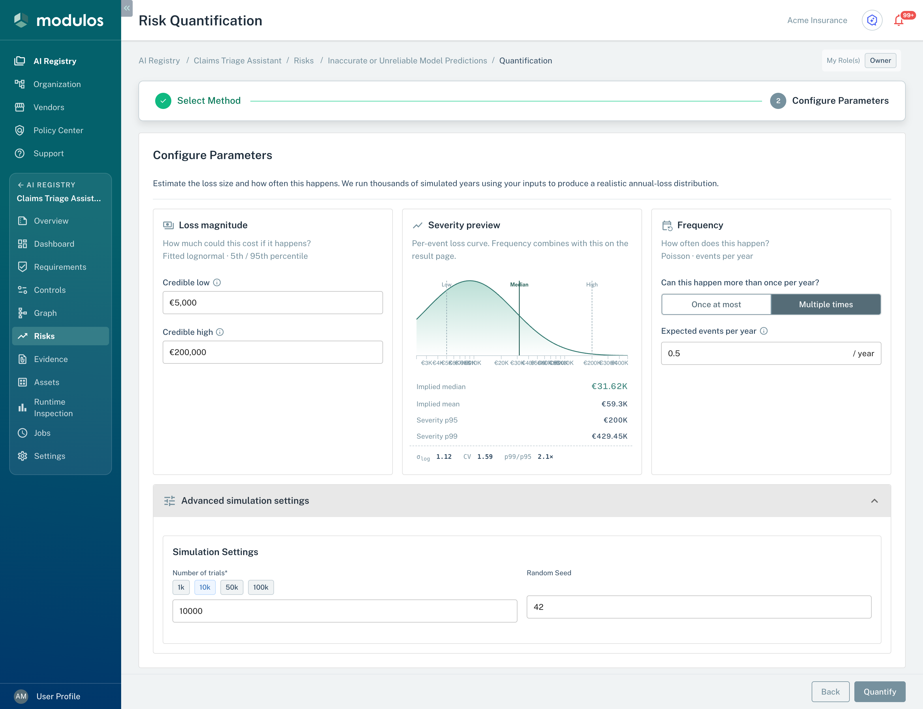
Monte Carlo Simulation asks for a loss range, a frequency, and simulation settings.
- Loss magnitude The loss of one incident, as a range from a credible low to a credible high value.
- Frequency Once at most asks for an annual probability. Multiple times asks for the expected events per year.
- Number of trials From 1 to 100,000 simulated years.
Result view
On the Current Analysis tab, a Monte Carlo run has four sections:
- The Simulation Results section: the Expected annual loss, the frequency, the standard error, and the run settings. A message shows when the expected annual loss is more than the calculated risk limit of the AI System. For this message, Modulos does not use a manual override of the limit.
- The Loss distribution section: a Risk threshold field and the probability that the annual loss is more than that threshold. A chart has the Distribution and Exceedance views. Three tiles show VaR and CVaR at the confidence level of the run, and Loss at p99. With the default confidence level of 95%, the tiles show VaR at 95% and CVaR at 95%. The default threshold is the calculated risk limit of the AI System. Without a limit, it is the 95th percentile of the annual loss.
- The Model assumptions section: what the run assumes about the incidents and the losses.
- The Advanced details section: the percentiles of the annual loss, the diagnostics of the run, and the raw parameters.
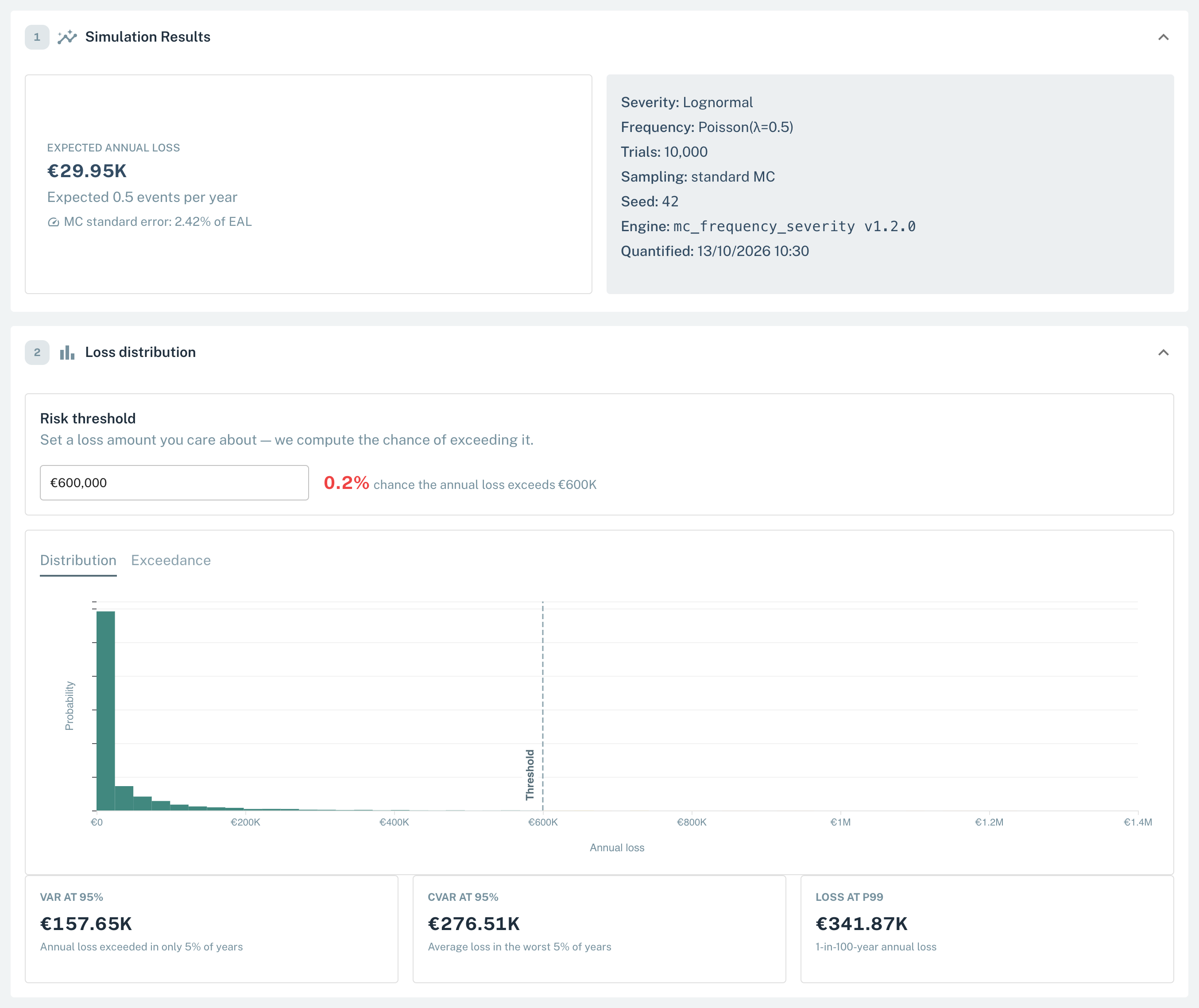
The result of a Monte Carlo Simulation shows the expected annual loss, the loss distribution, and the tail values.
- Expected annual loss The mean annual loss of all simulated years.
- Risk threshold Type a loss to see the probability that the annual loss is more than it.
- VaR at 95% The annual loss that only 5% of the simulated years are above.
Advanced Monte Carlo parameters
You can send these parameters in the montecarlo_frequency_severity request:
metrics: the metrics to calculate:EL,STD,QUANTILES,VAR,CVARalpha: the confidence level for VaR and CVaR, in(0, 1), default0.95collect_samples: include the samples in the output, defaultfalsemax_samples_output: the maximum number of samples in the output, default0antithetic: use antithetic sampling, defaultfalsestratified: use stratified sampling, defaultfalsehistogram_bins: the number of histogram bins, from 16 to 65,536, default2048allow_negative_severity: let the severity give negative values, defaultfalseallow_infinite_moments: let the simulation use very large draws above the standard caps, defaultfalsechunk_size: the number of trials in each simulation chunk, optionalsensitivity: the sensitivity configuration. This parameter is for experts and can change.
Risk Matrix
The Risk Matrix method changes ordinal inputs into money with a multiplication:
text
risk_score = likelihood_score × impact_score
quantified_value = risk_score × scaling_factor × frequency_multiplier
Use only with a calibrated mapping
Use Risk Matrix only when you have a calibration from your ordinal scores to monetary loss. A 5×5 matrix hides assumptions and causes category thinking. Use the output as a first estimate, and replace it with a better method when you can.
Inputs
likelihood_score: a number from 1 to 5.impact_score: a number from 1 to 5.scaling_factor: a multiplier that changes the score into money.frequency_multiplier: a multiplier for the number of times that the scenario occurs in your time basis.
UI fields
- A heat map. Select a cell to set Likelihood and Impact.
- Likelihood and Impact, from 1 to 5.
- Scaling Factor and Frequency Multiplier, more than 0.
The Risk Calculation Formula box shows the formula, the Risk Level, and the Score.
Result: the result shows the Likelihood, the Impact, and the Risk Score. The Analysis Breakdown section shows the inputs, the Risk Level, the Score, and the Financial Risk.
API payload
json
{
  "method": "risk_matrix",
  "likelihood_score": 3,
  "impact_score": 4,
  "scaling_factor": 100000,
  "frequency_multiplier": 1
}