

Appearance
Risk Quantification
What this is
Risk quantification changes risk statements into monetary outputs. You can then set priorities for mitigation and investment.
In Modulos, "quantified" means a numeric value. A qualitative 5×5 risk matrix is not quantification, and it can give incorrect priorities.
Where in Modulos
Quantification occurs at the level of the risk threat in each AI System:
AI System → Risks → [Risk] → Threat Vectors, then Quantify on the row of the threatAI System → Risks → [Risk] → [Threat], then Quantify or Recalculate on the Threat Quantification Detail page
The risk limits come from Organization → Risk Management → Risk Limits and AI System Risk Limits. They set the limit lines and the limit use, but they do not stop quantification. See Risk limits.
Who can do what
To start a quantification run, you must have the Owner role in the AI System. An organization role with full access to all AI Systems also lets you start runs: Organization Admin, Risk Manager, or Policy Manager. The other AI System roles can see the results.
How it works
Why not risk matrices
Qualitative matrices are weak at the points that are important to leaders:
- They do not divide a risk into rate and damage, so you cannot see which part a mitigation must decrease.
- They do not let you compare risks, AI Systems, or dates logically.
- Their colors and categories give an incorrect confidence.
Why money
Money is the unit because:
- it is the same unit for all types of risk
- it changes abstract losses (reputation, trust, the time to complete a mission) into terms that stakeholders know
- it connects directly to the risk appetite of the organization, which the organization shows through its budgets
The core model
Quantification gives the best results when it divides a risk into parts. Use the expected loss as the model:
text
Expected loss = Σ (rate × damage)- Rate: how frequently the threat becomes an incident, for a period or for a unit of work.
- Damage: the monetary loss for each incident, with all its costs: incident costs, indirect costs, and strategic costs.
An approximate estimate from clear assumptions is usually more useful than a qualitative rating. You can examine the assumptions and make them better.
- Define the threat One path with a clear cause of loss.
- Estimate rate How frequently it becomes an incident, with a clear denominator.
- Estimate damage All costs of each incident.
- Compute expected loss Get a monetary value that you can compare and budget.
Estimating rate
A clear structure makes the rate easy to estimate. Use a Fermi decomposition. Its purpose is clear assumptions that you can examine and make better.
text
Incidents/year = decisions/year × failure probability/decision × escalation fraction
Expected loss/year = incidents/year × loss/incident
Good practices:
- Use a denominator that you can defend, for example each deployment-year, each user-hour, or each 10,000 requests.
- Use telemetry and incident history when you have them. Use analogies when you do not.
- Write the assumptions down. Then other persons can examine them and make them better.
A useful property of numbers
An incorrect number can start a useful discussion. A statement such as "Your estimate assumes 10,000 requests per year, but telemetry shows 150,000" makes the model better. A statement such as "I disagree this is high risk" usually does not.
Estimating damage
The damage for each incident is usually a mix of these costs:
- incident cost: remediation, refunds, compensation, and legal and regulatory costs
- indirect cost: disruption of operations, workarounds, engineering time, and deals that you do not get
- strategic cost: damage to reputation and trust, market access, and limits in the future
It is hard to give a price to some losses, but it is possible. Use proxies that leaders know. Examples are revenue impact, customer loss, legal cost, remediation cost, and the cost of a release after its plan date.
How quantification works in the platform
In Modulos, quantification occurs at the level of the risk threat:
- Each AI System risk gets one or more risk threats when you add it. Each risk threat refers to one threat vector of the taxonomy.
- Each risk threat can have one or more quantification runs.
- Each run records the inputs, the outputs, a status, and one monetary value.
For example, an AI System risk with two risk threats and their runs:
AI System risk Risk threats Quantification runs
- Adversarial Attack Vulnerability The sum of its risk threats
- Direct Prompt Injection Counts the value of its newest run
- Newest run Quantified
- Older run Quantified
- Model extraction Counts 0
- Newest run Failed
- Older run Quantified
- Direct Prompt Injection Counts the value of its newest run
The newest run of a risk threat sets its status and its value. The value counts in the totals only when that run is Quantified. An older Quantified run does not count. For the rules, see How risk becomes a portfolio signal.
How to run quantification
- Open
AI System → Risksand select a risk. - On the Threat Vectors tab, select Quantify on the row of the threat.
- In Select Method, select a method card.
- Select Next.
- In Configure Parameters, enter the parameters of the method.
- Select Quantify.
Modulos starts the run and opens the Threat Quantification Detail page. The status of the threat is In Progress until the run is complete. A Risk Agent run can continue for some minutes.
If the threat has a previous run, the wizard fills in the method and the fields of the newest run. A run from the wizard uses the default values of the parameters that only the API sets. The Quantify and Recalculate buttons on the Threat Quantification Detail page also open the wizard. While the run on that page is In Progress, the button is not available.
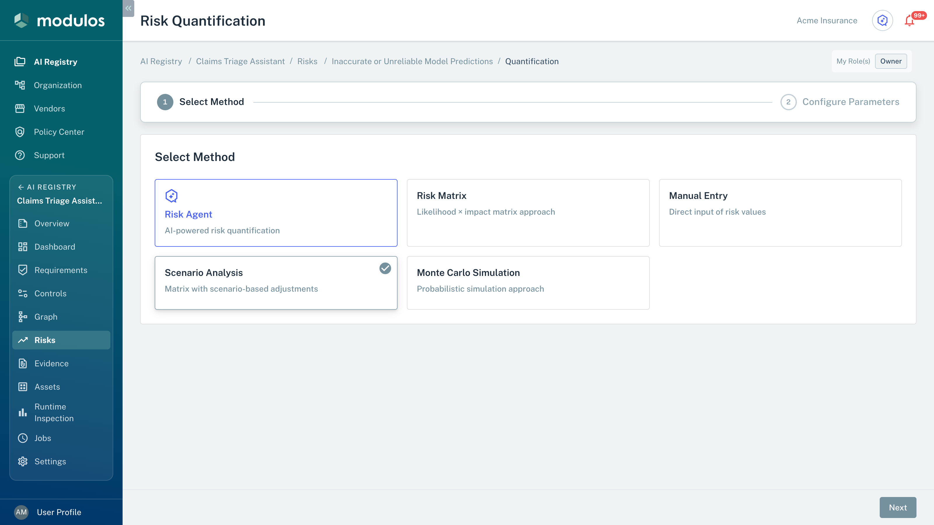
The quantification wizard starts with the selection of one of five methods.
- Select Method The first of the two steps of the wizard.
- Risk Agent The AI method. The other cards are the four numeric methods.
- Next Opens Configure Parameters for the selected method.
Run history and trends
The Threat Quantification Detail page (AI System → Risks → [Risk] → [Threat]) has three tabs. Users who can quantify also see Quantify, which shows Recalculate after the first run.
- Current Analysis: the newest run. The cards Quantified Value, Method, Status, and Quantified At show the value, the method, the status, and the date of the run. A panel below the cards shows the result of the method. Examples are the loss chart of a Monte Carlo Simulation and the scenarios of a Scenario Analysis. While a run is In Progress, the page shows Started At and waits for the result. For the panel of each method, see Quantification Methods.
- Risk Value Over Time: a chart of the value of the threat across its quantified runs, with a line for the risk limit. The cards above the chart are Current Value, Risk Change (%), and Utilization. Risk Change (%) compares the two newest runs with the status Quantified. After the first quantified run, it shows NEW. The Utilization card shows the current value as a percentage of the risk limit.
- Quantification History: a table of all runs of the threat, with Date, Method, Created By, Status, and Value. Use the Method and Status filters to show fewer runs. Select a row to open the run in a drawer. The drawer shows the cards and the method panel of that run. Previous and Next open the other runs, and Open in new tab opens the run on a full page.
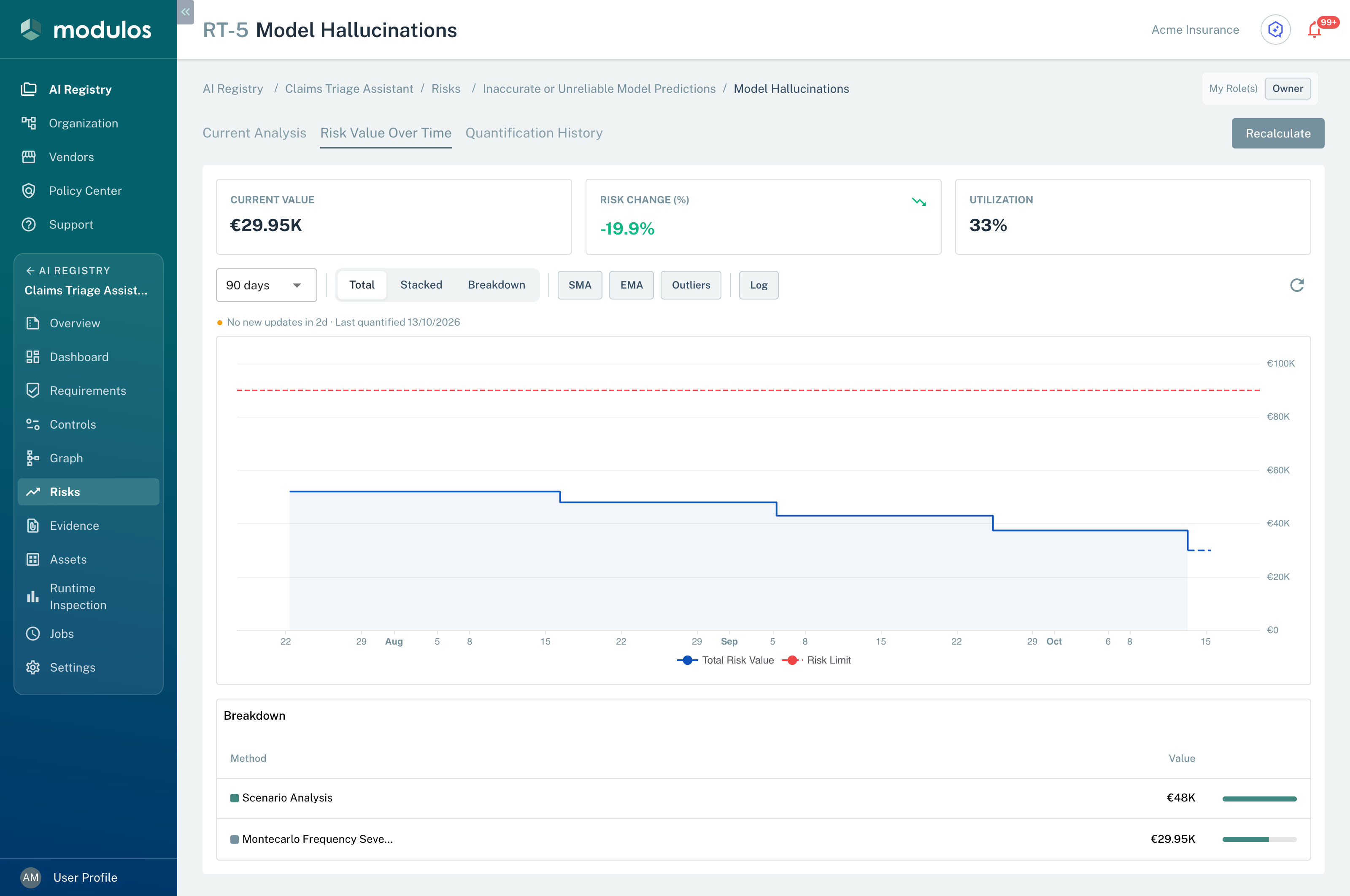
The Risk Value Over Time tab shows the value of a threat across its quantified runs.
- Risk Change (%) The change between the two newest quantified runs.
- Range The period of the chart. The buttons change the view.
- Risk Limit The limit of the risk, as a line.
The Risk Value Over Time charts have these controls:
- Range: 30 days, 90 days, 6 months, or 1 year. You can also zoom in the chart.
- The view: Total, the default, shows the sum. Stacked shows each part of the sum as an area. Breakdown shows each value as a point.
- SMA (simple moving average) and EMA (exponential moving average), with a Window in days.
- Outliers, with a Threshold in standard deviations.
- Log, for a logarithmic scale.
- A button that sets all controls back to their defaults.
Risk-level rollup chart
The same chart is on the page of each risk: AI System → Risks → [Risk] → Risk Value Over Time. In the Total view, it shows the sum of the risk threats and a line for the risk limit. It has no KPI cards. A table below the chart shows the value of each risk threat.
The Risks page of the AI System has the same chart for its risks. The Risk Overview tab of the organization has the same chart for the AI Systems.
Only "quantified" runs count
The charts show only runs with the status Quantified. Runs that are In Progress or Failed are in the Quantification History table, but not in the charts.
A chart keeps the value of the newest quantified run of each risk threat. When the newest run of a risk threat is In Progress or Failed, the totals count 0 for that risk threat. As a result, a chart and the totals can show different values.
Choosing a method
The wizard has five methods:
- Risk Agent: an AI agent makes a Fermi estimate and records its assumptions. See Risk Agent.
- Risk Matrix: changes a likelihood score and an impact score into money with a scaling factor and a frequency multiplier. Use it only with a calibrated mapping.
- Manual Entry: use it when you have a monetary estimate that you can defend.
- Scenario Analysis: use it to give a structure to your assumptions with the Best Case, Base Case, and Worst Case scenarios.
- Monte Carlo Simulation: use it when you want a probabilistic model and can defend its inputs.
Start simple, then add rigor
A complex model does not make weak inputs better. If you do not have incident data, start with Scenario Analysis and clear assumptions. Use Monte Carlo Simulation when you can defend your estimates of loss and frequency to stakeholders.
What Modulos stores
Each quantification run records:
- the method
- the input parameters and the output values
- the status, the user who started the run, and the date
- one monetary value for the totals
Calibration
Apply quantification as a continuous loop:
- record incidents and near misses from the first day
- compare the estimates with the actual results at regular intervals
- change the assumptions, the taxonomy, and the methods when the conditions change
Without feedback, the numbers become an incorrect precision.
When quantification fails
Quantification can be systematically incorrect when analogies do not apply, when experts share the same bias, or when the domain is new. The correction is calibration: compare previous estimates with actual results, and change your assumptions and your taxonomy.
Important considerations
Quantification runs with all limit configurations. But the limit use and the limit lines are correct only when the limits agree. Modulos shows warnings while you edit limits that do not agree. For the rules, see Risk limits.